In mathematics, a Gaussian function (named after Carl Friedrich Gauss) is a function of the form:

for arbitrary real constants a, b, c, d.
The graph of a Gaussian is a characteristic symmetric “bell curve” shape that quickly falls off towards zero. The parameter a is the height of the curve’s peak, b is the position of the center of the peak, andc (the standard deviation) controls the width of the “bell”.
Gaussian functions are widely used in statistics where they describe the normal distributions, in signal processing where they serve to define Gaussian filters, in image processing where two-dimensional Gaussians are used for Gaussian blurs, and in mathematics where they are used to solve heat equations and diffusion equations and to define the Weierstrass transform.
Properties
Gaussian functions arise by applying the exponential function to a general quadratic function. The Gaussian functions are thus those functions whose logarithm is a quadratic function.
The parameter c is related to the full width at half maximum (FWHM) of the peak according to

Alternatively, the parameter c can be interpreted by saying that the two inflection points of the function occur at x = b − c and x = b + c.
The full width at tenth of maximum (FWTM) for a Gaussian could be of interest and is

Gaussian functions are analytic, and their limit as x → ∞ is 0.
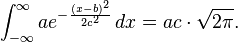
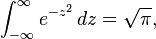
Gaussian functions are among those functions that are elementary but lack elementary antiderivatives; the integral of the Gaussian function is the error function. Nonetheless their improper integrals over the whole real line can be evaluated exactly, using theGaussian integral
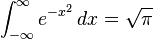
and one obtains
This integral is 1 if and only if a = 1/(c√(2π)), and in this case the Gaussian is the probability density function of a normally distributed random variable with expected value μ = b and variance σ2 = c2:
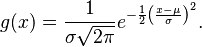
These Gaussians are plotted in the accompanying figure.
Gaussian functions centered at zero minimize the Fourier uncertainty principle.
The product of two Gaussian functions is a Gaussian (warning: the product of two Gaussian probability density functions is not in general a Gaussian pdf), and the convolution of two Gaussian functions is also a Gaussian, with std. deviation being the quadratic mean of the original std. deviations: 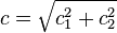 .
.
Taking the Fourier transform (unitary, angular frequency convention) of a Gaussian function with parameters a, b = 0 and c yields another Gaussian function, with parameters  , b = 0 and
  .[3] So in particular the Gaussian functions with b = 0 and c =
  are kept fixed by the Fourier transform (they are eigenfunctions of the Fourier transform with eigenvalue 1).
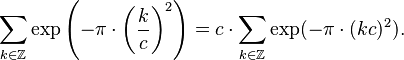
The fact that the Gaussian function is an eigenfunction of the Continuous Fourier transform allows us to derive the following interesting identity from the Poisson summation formula:
Integral of a Gaussian function
The integral of an arbitrary Gaussian function is
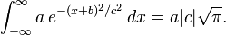
An alternative form is

where f must be strictly positive for the integral to converge.
Proof[edit]
The integral
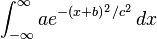
for some real constants a, b, c > 0 can be calculated by putting it into the form of a Gaussian integral. First, the constant a can simply be factored out of the integral. Next, the variable of integration is changed from x to y = x + b.
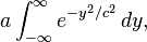
and then to 

Then, using the Gaussian integral identity
we have

Two-dimensional Gaussian function

Gaussian curve with a 2-dimensional domain
In two dimensions, the power to which e is raised in the Gaussian function is any negative-definite quadratic form. Consequently, the level sets of the Gaussian will always be ellipses.
A particular example of a two-dimensional Gaussian function is
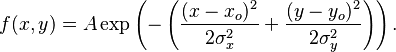
Here the coefficient A is the amplitude, xo,yo is the center and σx, σy are the x and y spreads of the blob. The figure on the right was created using A = 1, xo = 0, yo = 0, σx = σy = 1.
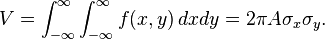
The volume under the Gaussian function is given by
In general, a two-dimensional elliptical Gaussian function is expressed as

where the matrix
![\left[\begin{matrix} a & b \\ b & c \end{matrix}\right]](http://upload.wikimedia.org/math/5/3/f/53f022c87448b5afdf1062ec965f4db7.png)
Using this formulation, the figure on the right can be created using A = 1, (xo, yo) = (0, 0), a = c = 1/2, b = 0.
Meaning of parameters for the general equation
For the general form of the equation the coefficient A is the height of the peak and (xo, yo) is the center of the blob.
If we set

then we rotate the blob by a clockwise angle  (for counterclockwise rotation invert the signs in the b coefficient). This can be seen in the following examples:
 |


Using the following Octave code one can easily see the effect of changing the parameters
A = 1;
x0 = 0; y0 = 0;

sigma_x = 1;
sigma_y = 2;

for theta = 0:pi/100:pi
    a = cos(theta)^2/2/sigma_x^2 + sin(theta)^2/2/sigma_y^2;
    b = -sin(2*theta)/4/sigma_x^2 + sin(2*theta)/4/sigma_y^2 ;
    c = sin(theta)^2/2/sigma_x^2 + cos(theta)^2/2/sigma_y^2;

    [X, Y] = meshgrid(-5:.1:5, -5:.1:5);
    Z = A*exp( - (a*(X-x0).^2 + 2*b*(X-x0).*(Y-y0) + c*(Y-y0).^2)) ;
    surf(X,Y,Z);shading interp;view(-36,36);axis equal;drawnow
end
Such functions are often used in image processing and in computational models of visual system function—see the articles on scale space and affine shape adaptation.
Also see multivariate normal distribution.
Multi-dimensional Gaussian function
In an  -dimensional space a Gaussian function can be defined as
where  is a column of coordinates,
  is a positive-definite
  matrix, and
  denotes transposition.
The integral of this Gaussian function over the whole -dimensional space is given as
It can be easily calculated by diagonalizing the matrix and changing the integration variables to the eigenvectors of .
More generally a shifted Gaussian function is defined as

where 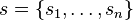 is the shift vector and the matrix can be assumed to be symmetric,
  , and positive-definite. The following integrals with this function can be calculated with the same technique,


Gaussian profile estimation
A number of fields such as stellar photometry, Gaussian beam characterization, and emission/absorption line spectroscopy work with sampled Gaussian functions and need to accurately estimate the height, position, and width parameters of the function. These are  ,
,  , and
, and  for a 1D Gaussian function, ,
  , and
, and  for a 2D Gaussian function. The most common method for estimating the profile parameters is to take the logarithm of the data and fit a parabola to the resulting data set.[4] While this provides a simpleleast squares fitting procedure, the resulting algorithm is biased by excessively weighting small data values, and this can produce large errors in the profile estimate. One can partially compensate for this through weighted least squares estimation, in which the small data values are given small weights, but this too can be biased by allowing the tail of the Gaussian to dominate the fit. In order to remove the bias, one can instead use an iterative procedure in which the weights are updated at each iteration (see Iteratively reweighted least squares).[4]
Once one has an algorithm for estimating the Gaussian function parameters, it is also important to know how accurate those estimates are. While an estimation algorithm can provide numerical estimates for the variance of each parameter (i.e. the variance of the estimated height, position, and width of the function), one can use Cramér–Rao bound theory to obtain an analytical expression for the lower bound on the parameter variances, given some assumptions about the data.[5][6]
- The noise in the measured profile is either i.i.d. Gaussian, or the noise is Poisson-distributed.
- The spacing between each sampling (i.e. the distance between pixels measuring the data) is uniform.
- The peak is “well-sampled”, so that less than 10% of the area or volume under the peak (area if a 1D Gaussian, volume if a 2D Gaussian) lies outside the measurement region.
- The width of the peak is much larger than the distance between sample locations (i.e. the detector pixels must be at least 5 times smaller than the Gaussian FWHM).
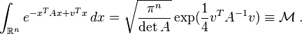
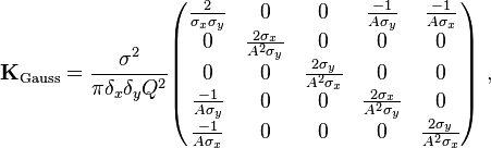
When these assumptions are satisfied, the following covariance matrix K applies for the 1D profile parameters , , and under i.i.d. Gaussian noise and under Poisson noise:[5]

where  is the width of the pixels used to sample the function,
  is the quantum efficiency of the detector, and
  indicates the standard deviation of the measurement noise. Thus, the individual variances for the parameters are, in the Gaussian noise case,
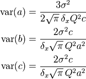
and in the Poisson noise case,
For the 2D profile parameters giving the amplitude , position , and width of the profile, the following covariance matrices apply:[6]

where the individual parameter variances are given by the diagonal elements of the covariance matrix.
Discrete Gaussian

The discrete Gaussian kernel(black, dashed), compared with thesampled Gaussian kernel (red, solid) for scales 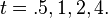
One may ask for a discrete analog to the Gaussian; this is necessary in discrete applications, particularly digital signal processing. A simple answer is to sample the continuous Gaussian, yielding the sampled Gaussian kernel. However, this discrete function does not have the discrete analogs of the properties of the continuous function, and can lead to undesired effects, as described in the article scale space implementation.
An alternative approach is to use discrete Gaussian kernel:[7]
where  denotes the modified Bessel functions of integer order.
This is the discrete analog of the continuous Gaussian in that it is the solution to the discrete diffusion equation (discrete space, continuous time), just as the continuous Gaussian is the solution to the continuous diffusion equation.[8]
Applications
Gaussian functions appear in many contexts in the natural sciences, the social sciences, mathematics, and engineering. Some examples include:
- In statistics and probability theory, Gaussian functions appear as the density function of the normal distribution, which is a limiting probability distribution of complicated sums, according to the central limit theorem.
- Gaussian functions are the Green’s function for the (homogeneous and isotropic) diffusion equation (and, which is the same thing, to the heat equation), a partial differential equation that describes the time evolution of a mass-density under diffusion. Specifically, if the mass-density at time t=0 is given by a Dirac delta, which essentially means that the mass is initially concentrated in a single point, then the mass-distribution at time t will be given by a Gaussian function, with the parameter a being linearly related to 1/√t and c being linearly related to √t. More generally, if the initial mass-density is φ(x), then the mass-density at later times is obtained by taking theconvolution of φ with a Gaussian function. The convolution of a function with a Gaussian is also known as a Weierstrass transform.
- A Gaussian function is the wave function of the ground state of the quantum harmonic oscillator.
- The molecular orbitals used in computational chemistry can be linear combinations of Gaussian functions called Gaussian orbitals (see also basis set (chemistry)).
- Mathematically, the derivatives of the Gaussian function can be represented using Hermite functions. The n-th derivative of the Gaussian is the Gaussian function itself multiplied by the n-th Hermite polynomial, up to scale.
- Consequently, Gaussian functions are also associated with the vacuum state in quantum field theory.
- Gaussian beams are used in optical and microwave systems.
- In scale space representation, Gaussian functions are used as smoothing kernels for generating multi-scale representations in computer vision and image processing. Specifically, derivatives of Gaussians (Hermite functions) are used as a basis for defining a large number of types of visual operations.
- Gaussian functions are used to define some types of artificial neural networks.
- In fluorescence microscopy a 2D Gaussian function is used to approximate the Airy disk, describing the intensity distribution produced by a point source.
- In signal processing they serve to define Gaussian filters, such as in image processing where 2D Gaussians are used for Gaussian blurs. In digital signal processing, one uses a discrete Gaussian kernel, which may be defined by sampling a Gaussian, or in a different way.
- In geostatistics they have been used for understanding the variability between the patterns of a complex training image. They are used with kernel methods to cluster the patterns in the feature space.[9]